Effects of Sewage

Oxygen Sag Curve

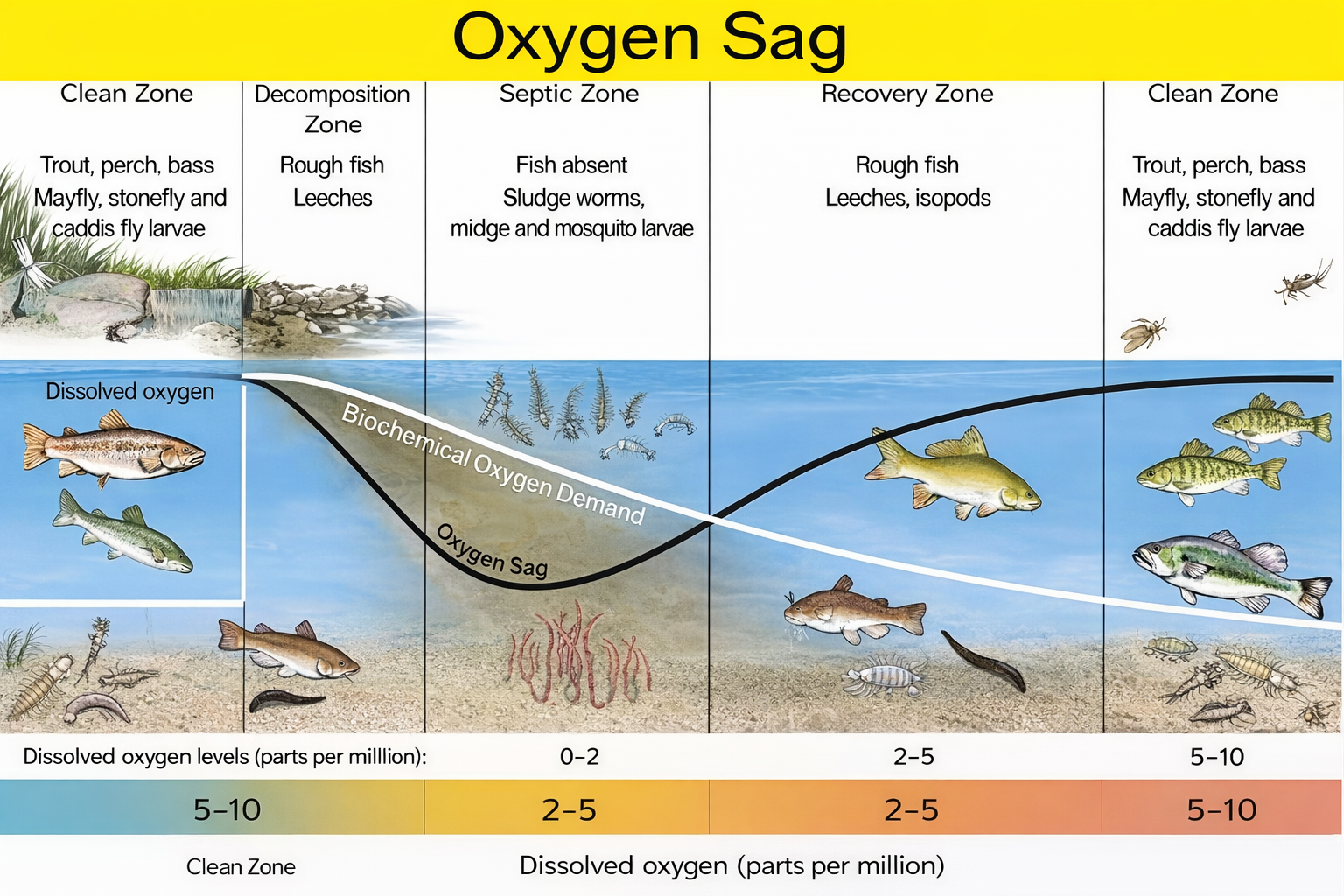
By far the most important characteristic determining the quality of a river or stream is its dissolved oxygen, DO (measured in mg/L).

While saturation is rarely achieved, a stream can nonetheless be considered healthy as long as its dissolved oxygen DO exceed 5 mg/L.

Below 5 mg/L, most fish, especially the more desirable species such as trout, do not survive.

The discharge of a sewage effluent in a stream produces a biochemical oxygen demand. This oxygen demand causes an oxygen deficit, or oxygen shortage. The greater the oxygen deficit, the greater the rate of natural oxygen replenishment from the atmosphere into the stream.

Two concurrent processes of oxygen consumption and oxygen replenishment produce an oxygen sag curve.

An oxygen sag curve graphically represents the changes in dissolved oxygen levels in a body of water, typically a river or stream, following the addition of organic pollutants. 

An oxygen sag curve is a graph that shows how the concentration of dissolved oxygen in a body of water changes over distance from a point of pollution. The curve is created by plotting the concentration of dissolved oxygen against the distance downstream from a sewage outlet or other pollutant source. 

The curve shows a sag, or drop, in dissolved oxygen levels due to the increased demand for oxygen by microorganisms that consume oxygen as they decompose organic pollutants. The curve then recovers downstream as the rate of oxygen replenishment increases. 

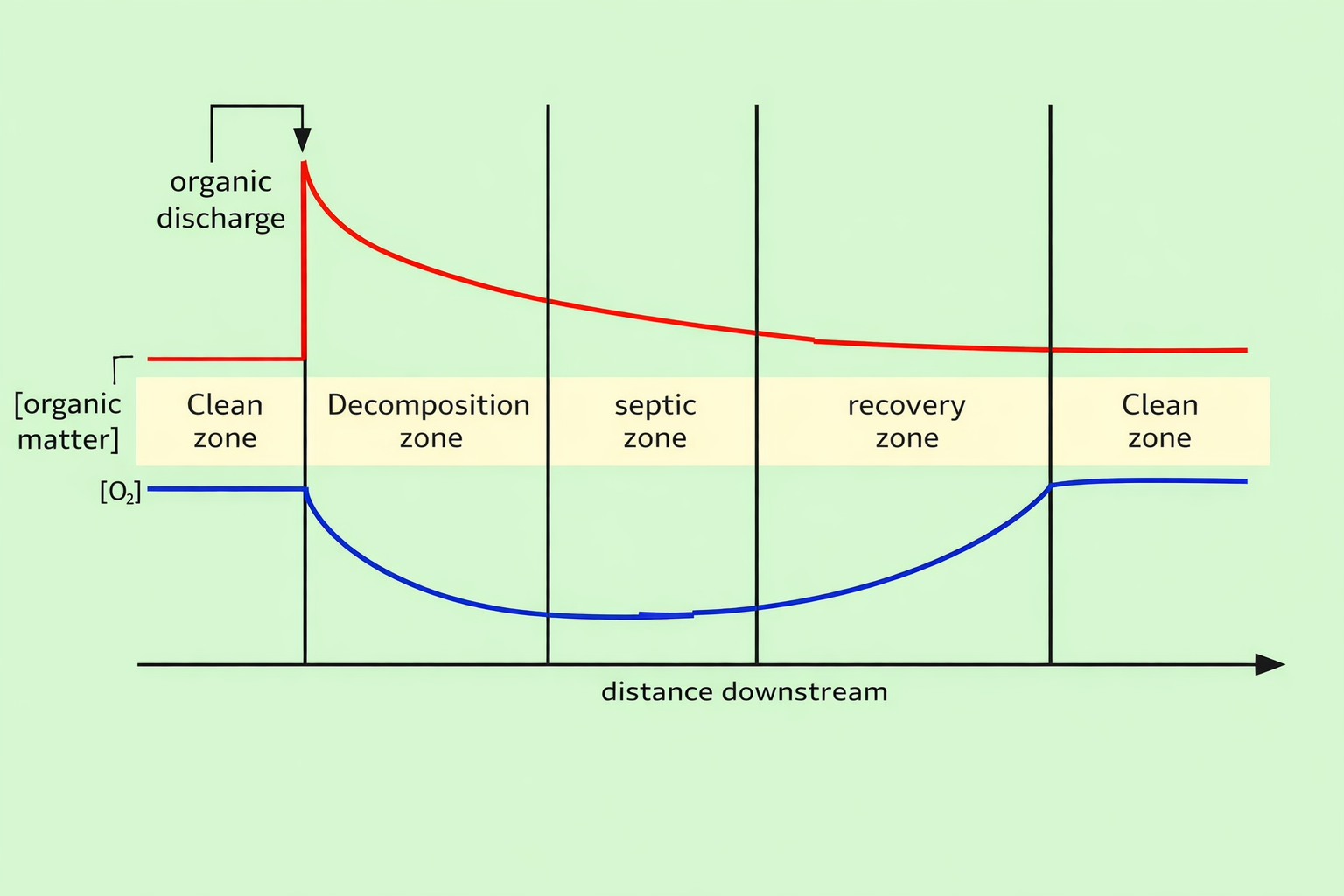
The oxygen sag curve shows different zones as the water flows from the pollution source, including: 

• Clean zone: The dissolved oxygen level is high
• Decomposition zone: The dissolved oxygen level drops
• Septic zone: The dissolved oxygen level drops
• Recovery zone: The dissolved oxygen level recovers
• Final clean zone: The dissolved oxygen level returns to high

Streeter–Phelps Equation

The Streeter–Phelps equation derived by H. W. Streeter, a sanitary engineer, and Erle B. Phelps a 

consultant for the U.S. Public Health Service, in 1925, based on field data from the Ohio River.

The Streeter – Phelps equation is used in the study of water pollution and as a water quality monitoring tool. The Streeter-Phelps equation is used to set discharge limits for sewage by calculating the potential “oxygen sag” in a river downstream from a discharge point, allowing regulators to determine the maximum amount of biochemical oxygen demand (BOD) that can be released without causing critically low dissolved oxygen levels, which are harmful to aquatic life; essentially, it helps set limits to ensure the river can adequately reoxygenate after receiving the sewage effluent. 

Modeling the Oxygen Sag Curve:

The equation mathematically describes the decline in dissolved oxygen concentration (due to organic matter decomposition) followed by a recovery as the water reoxygenates downstream from a pollution source, creating a “sag curve.”. 

The equation takes into account factors like the initial dissolved oxygen concentration, the rate of deoxygenation (related to BOD), the rate of reaeration (dependent on water velocity and turbulence), water temperature, and stream characteristics. 

By analyzing the calculated sag curve, regulators can identify the “critical point” where the dissolved oxygen concentration reaches its lowest level, allowing them to set discharge limits that prevent this level from falling below a predetermined standard for aquatic life protection. 

How it works:

Environmental data like stream flow, temperature, BOD concentration of the sewage effluent, and the deoxygenation and reaeration rates are inputted into the Streeter-Phelps equation. 

The equation calculates the dissolved oxygen concentration at different distances downstream from the discharge point, creating the oxygen sag curve. 

By comparing the calculated oxygen levels to water quality standards, regulators can set discharge limits for the sewage treatment plant to ensure the dissolved oxygen in the river remains within acceptable levels. 

A dissolved oxygen level of 4 mg/L is generally recommended. 

When the level drops below 2.0 mg/L, some aquatic animals may become distressed or die from suffocation. The Streeter Phelps equation calculates the dissolved oxygen concentration at different distances downstream from the discharge point, creating the oxygen sag curve. 

By comparing the calculated oxygen levels to water quality standards, regulators can set discharge limits for the sewage treatment plant to ensure the dissolved oxygen in the river remains within acceptable levels. 

“BOD reduction rate constant” the constant “k”

The Streeter Phelps equation also calculates “BOD reduction rate constant” the constant “k”, that represents the rate at which Biochemical Oxygen Demand (BOD)decreases over time in a water body, essentially indicating how quickly organic matter is being decomposed by microorganisms and consuming oxygen in the process; it is typically expressed as a value per unit time (e.g., per day) and is used in calculations to predict the oxygen depletion in a water system based on its initial BOD level.

The BOD rate constant is high for the raw sewage (K = 0.35 -0.7 per day) and low for the treated sewage 

(K = 0.12 – 0.23 per day), 

To calculate BOD (Biochemical Oxygen Demand) using the decay constant, you use the formula:

BOD(t) = L * (1 – e^(-k * t)) where: 

BOD(t): is the BOD at a specific time “t”.

L: is the initial BOD 

k: is the BOD decay constant 

t: is the time elapsed.

BOD(t) = L0 * e^(-k * t)

BOD(5 days) = 60 mg/L * e^(- 0.62 * 5 days) 

BOD(5 days) = 60 mg/L e^ 3.4

BOD(5 days) = 60 mg/L e^ 3.4 * 5 – 17

BOD(5 days) = 60 mg/L = 60 – 17 = 43

BOD(5 days) = 43 mg/l

Activity Oxygen Sag Curve 

Directions

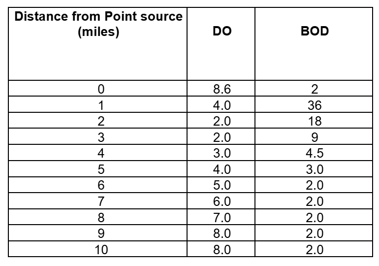
1. Enter the data from the table into an Excel spread sheet.
2. Plot the DO and BOD levels versus the distance downstream of a point source of pollution.